Tidy data

Variables, values, and observations

In the exploratory data analysis primer, we proposed three definitions that are useful for data science:

A variable is a quantity, quality, or property that you can measure.
A value is the state of a variable when you measure it. The value of a variable may change from measurement to measurement.
An observation is a set of measurements that are made under similar conditions (you usually make all of the measurements in an observation at the same time and on the same object). An observation will contain several values, each associated with a different variable. I’ll sometimes refer to an observation as a case or data point.

These definitions are tied to the concept of tidy data. To see how, let’s apply the definitions to some real data.

Quiz 1: What are the variables?

table1

# A tibble: 6 × 4
  country      year  cases population
  <chr>       <dbl>  <dbl>      <dbl>
1 Afghanistan  1999    745   19987071
2 Afghanistan  2000   2666   20595360
3 Brazil       1999  37737  172006362
4 Brazil       2000  80488  174504898
5 China        1999 212258 1272915272
6 China        2000 213766 1280428583

What are the variables in the dataset above? Check all that apply.

Quiz 2: What are the variables?

Now consider this dataset. Does it contain the same variables?

table2

# A tibble: 12 × 4
   country      year type            count
   <chr>       <dbl> <chr>           <dbl>
 1 Afghanistan  1999 cases             745
 2 Afghanistan  1999 population   19987071
 3 Afghanistan  2000 cases            2666
 4 Afghanistan  2000 population   20595360
 5 Brazil       1999 cases           37737
 6 Brazil       1999 population  172006362
 7 Brazil       2000 cases           80488
 8 Brazil       2000 population  174504898
 9 China        1999 cases          212258
10 China        1999 population 1272915272
11 China        2000 cases          213766
12 China        2000 population 1280428583

Does the data above contain information on country, year, cases, and population?

The shapes of data

These data sets reveal something important: you can reorganize the same set of variables, values, and observations in many different ways.

It’s not hard to do. If you run the code chunks below, you can see the same data displayed in three more ways.

Interactive editor

Interactive editor

Interactive editor

Tidy data

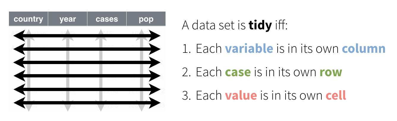
Data can come in a variety of formats, but one format is easier to use in R than the others. This format is known as tidy data. A data set is tidy if:

Each variable is in its own column
Each observation is in its own row
Each value is in its own cell (this follows from #1 and #2)

Among our tables above, only table1 is tidy.

table1

# A tibble: 6 × 4
  country      year  cases population
  <chr>       <dbl>  <dbl>      <dbl>
1 Afghanistan  1999    745   19987071
2 Afghanistan  2000   2666   20595360
3 Brazil       1999  37737  172006362
4 Brazil       2000  80488  174504898
5 China        1999 212258 1272915272
6 China        2000 213766 1280428583

Extracting variables

To see why tidy data is easier to use, consider a basic task. Each code chunk below extracts the values of the cases variable as a vector and computes the mean of the variable. One uses a tidy table, table1:

table1

# A tibble: 6 × 4
  country      year  cases population
  <chr>       <dbl>  <dbl>      <dbl>
1 Afghanistan  1999    745   19987071
2 Afghanistan  2000   2666   20595360
3 Brazil       1999  37737  172006362
4 Brazil       2000  80488  174504898
5 China        1999 212258 1272915272
6 China        2000 213766 1280428583

mean(table1$cases)

[1] 91276.67

The other uses an untidy table, table2:

table2

# A tibble: 12 × 4
   country      year type            count
   <chr>       <dbl> <chr>           <dbl>
 1 Afghanistan  1999 cases             745
 2 Afghanistan  1999 population   19987071
 3 Afghanistan  2000 cases            2666
 4 Afghanistan  2000 population   20595360
 5 Brazil       1999 cases           37737
 6 Brazil       1999 population  172006362
 7 Brazil       2000 cases           80488
 8 Brazil       2000 population  174504898
 9 China        1999 cases          212258
10 China        1999 population 1272915272
11 China        2000 cases          213766
12 China        2000 population 1280428583

mean(table2$count[c(1, 3, 5, 7, 9, 11)])

[1] 91276.67

Which line of code is easier to write? Which line could you write if you’ve only looked at the first row of the data?

Reusing code

Not only is the code for table1 easier to write, it is easier to reuse. To see what I mean, modify the code chunks below to compute the mean of the population variable for each table.

First with table1:

table1

# A tibble: 6 × 4
  country      year  cases population
  <chr>       <dbl>  <dbl>      <dbl>
1 Afghanistan  1999    745   19987071
2 Afghanistan  2000   2666   20595360
3 Brazil       1999  37737  172006362
4 Brazil       2000  80488  174504898
5 China        1999 212258 1272915272
6 China        2000 213766 1280428583

Interactive editor
Solution

mean(table1$population)

Then with table2:

table2

# A tibble: 12 × 4
   country      year type            count
   <chr>       <dbl> <chr>           <dbl>
 1 Afghanistan  1999 cases             745
 2 Afghanistan  1999 population   19987071
 3 Afghanistan  2000 cases            2666
 4 Afghanistan  2000 population   20595360
 5 Brazil       1999 cases           37737
 6 Brazil       1999 population  172006362
 7 Brazil       2000 cases           80488
 8 Brazil       2000 population  174504898
 9 China        1999 cases          212258
10 China        1999 population 1272915272
11 China        2000 cases          213766
12 China        2000 population 1280428583

Interactive editor
Solution

mean(table2$count[c(2, 4, 6, 8, 10, 12)])

Again table1 is easier to work with; you only need to change the name of the variable that you wish to extract. Code like this is easier to generalize to new datasets (if they are tidy) and easier to automate with a function.

Let’s look at one more advantage.

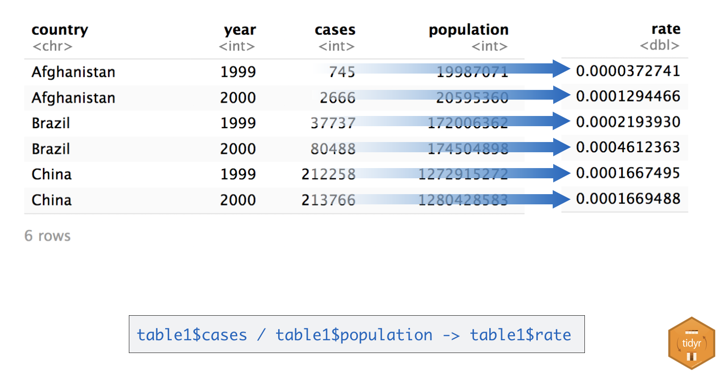
Calculations

Suppose you would like to compute the ratios of cases to population for each country and each year. To do this, you need to ensure that the correct value of cases is paired with the correct value of population when you do the calculation.

Again, this is hard to do with untidy table2:

table2

# A tibble: 12 × 4
   country      year type            count
   <chr>       <dbl> <chr>           <dbl>
 1 Afghanistan  1999 cases             745
 2 Afghanistan  1999 population   19987071
 3 Afghanistan  2000 cases            2666
 4 Afghanistan  2000 population   20595360
 5 Brazil       1999 cases           37737
 6 Brazil       1999 population  172006362
 7 Brazil       2000 cases           80488
 8 Brazil       2000 population  174504898
 9 China        1999 cases          212258
10 China        1999 population 1272915272
11 China        2000 cases          213766
12 China        2000 population 1280428583

table2$count[c(1, 3, 5, 7, 9, 11)] / table2$count[c(2, 4, 6, 8, 10, 12)]

[1] 0.0000372741 0.0001294466 0.0002193930 0.0004612363 0.0001667495
[6] 0.0001669488

But it is easy to do with tidy table1. Give it a try below:

table1

# A tibble: 6 × 4
  country      year  cases population
  <chr>       <dbl>  <dbl>      <dbl>
1 Afghanistan  1999    745   19987071
2 Afghanistan  2000   2666   20595360
3 Brazil       1999  37737  172006362
4 Brazil       2000  80488  174504898
5 China        1999 212258 1272915272
6 China        2000 213766 1280428583

Interactive editor
Solution

table1$cases / table1$population

These small differences may seem petty, but they add up over the course of a data analysis, stealing time and inviting mistakes.

Tidy data and R

The tidy data format works so well for R because it aligns the structure of your data with the mechanics of R:

R stores each data frame as a list of column vectors, which makes it easy to extract a column from a data frame as a vector. Tidy data places each variable in its own column vector, which makes it easy to extract all of the values of a variable to compute a summary statistic, or to use the variable in a computation.
R computes many functions and operations in a vectorized fashion, matching the first values of each vector of input to compute the first result, matching the second values of each input to compute the second result, and so on. Tidy data ensures that R will always match values with other values from the same operation whenever vector inputs are drawn from the same table.

As a result, most functions in R—and every function in the tidyverse—will expect your data to be organized into a tidy format. (You may have noticed above that we could use {dplyr} functions to work on table1, but not on table2).

Recap

“Data comes in many formats, but R prefers just one: tidy data.”

— Garrett Grolemund

A data set is tidy if:

Each variable is in its own column
Each observation is in its own row
Each value is in its own cell (this follows from #1 and #2)

Now that you know what tidy data is, what can you do about untidy data?

Next topic