Legends
Customizing a legend
The last piece of a {ggplot2} graph to customize is the legend. When it comes to legends, you can customize the:
- position of the legend within the graph
- the “type” of the legend, or whether a legend appears at all
- the title and labels in the legend
Customizing legends is a little more chaotic than customizing other parts of the graph, because the information that appears in a legend comes from several different places.
Positions
To change the position of a legend in a {ggplot2} graph add one of the below to your plot call:
+ theme(legend.position = "bottom")+ theme(legend.position = "top")+ theme(legend.position = "left")+ theme(legend.position = "right")(the default)
Try this now. Move the legend in p_cont to the bottom of the graph.
p_cont + theme(legend.position = "bottom")Good job! If you move the legend to the top or bottom of the plot, {ggplot2} will reogranize the orientation of the legend from vertical to horizontal.
theme() vs. themes
Theme functions like theme_grey() and theme_bw() also adjust the legend position (among all of the other details they orchestrate). So if you use theme(legend.position = "bottom") in your plots, be sure to add it after any theme_ functions you call, like this
If you do this, ggplot2 will apply all of the settings of theme_bw(), and then overwrite the legend position setting to “bottom” (instead of vice versa).
Types
You may have noticed that color and fill legends take two forms. If you map color (or fill) to a discrete variable, the legend will look like a standard legend. This is the case for the bottom legend below.
If you map color (or fill) to a continuous legend, your legend will look like a colorbar. This is the case in the top legend below. The color bar helps convey the continuous nature of the variable.
p_legend <- ggplot(data = mpg) +
  geom_jitter(mapping = aes(x = displ, y = hwy, color = class, fill = hwy),
              shape = 21, size = 3, stroke = 1) +
  theme_bw()

p_legend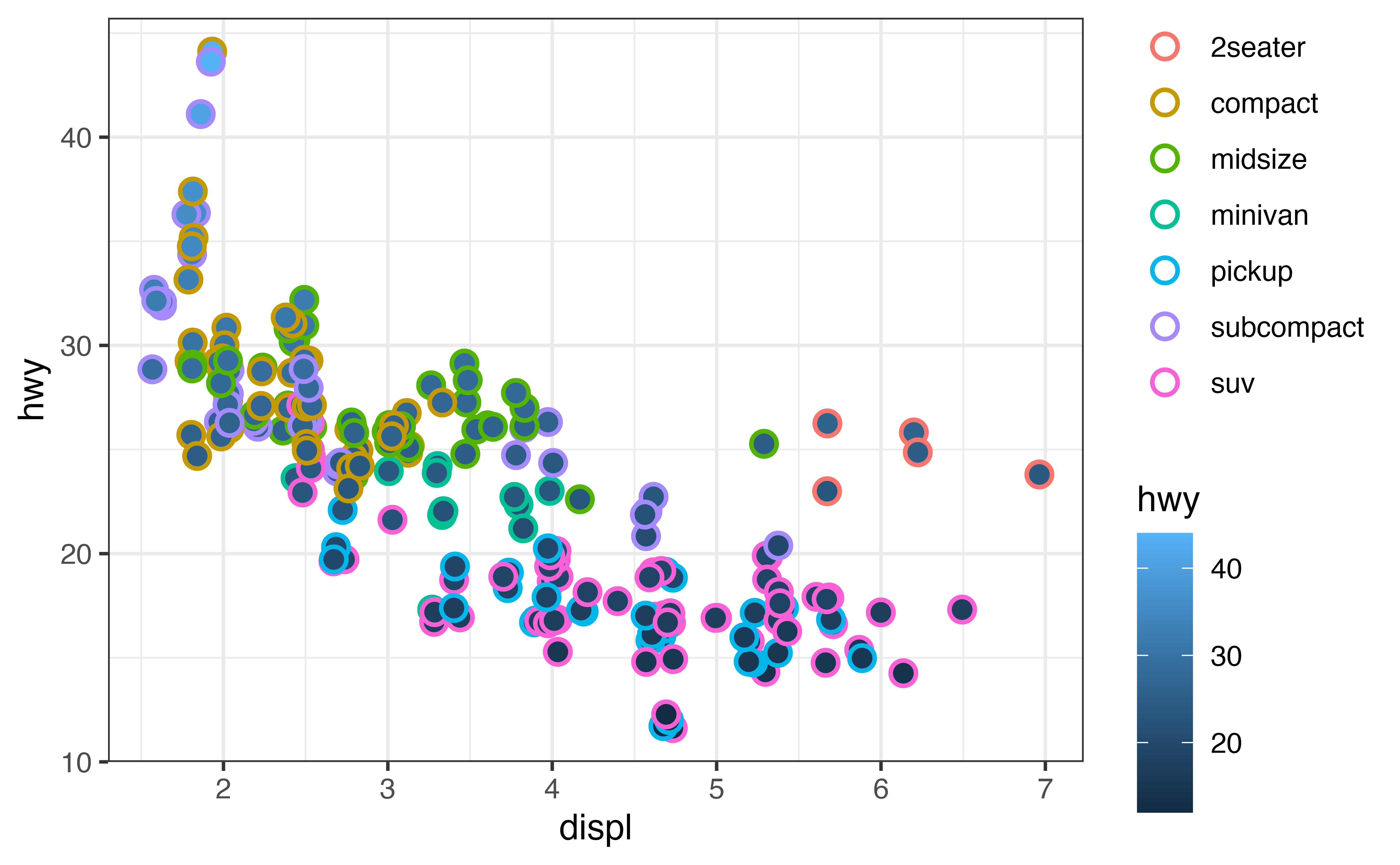
Changing type
You can use the guides() function to change the type or presence of each legend in the plot. To use guides(), type the name of the aesthetic whose legend you want to alter as and argument name. Then set it to one of
"legend": to force a legend to appear as a standard legend instead of a colorbar"colorbar": to force a legend to appear as a colorbar instead of a standard legend. Note: this can only be used when the legend can be printed as a colorbar (in which case the default will be colorbar)."none": to remove the legend entirely. This is useful when you have redundant aesthetic mappings, but it may make your plot indecipherable otherwise.
p_legend + guides(fill = "legend", color = "none")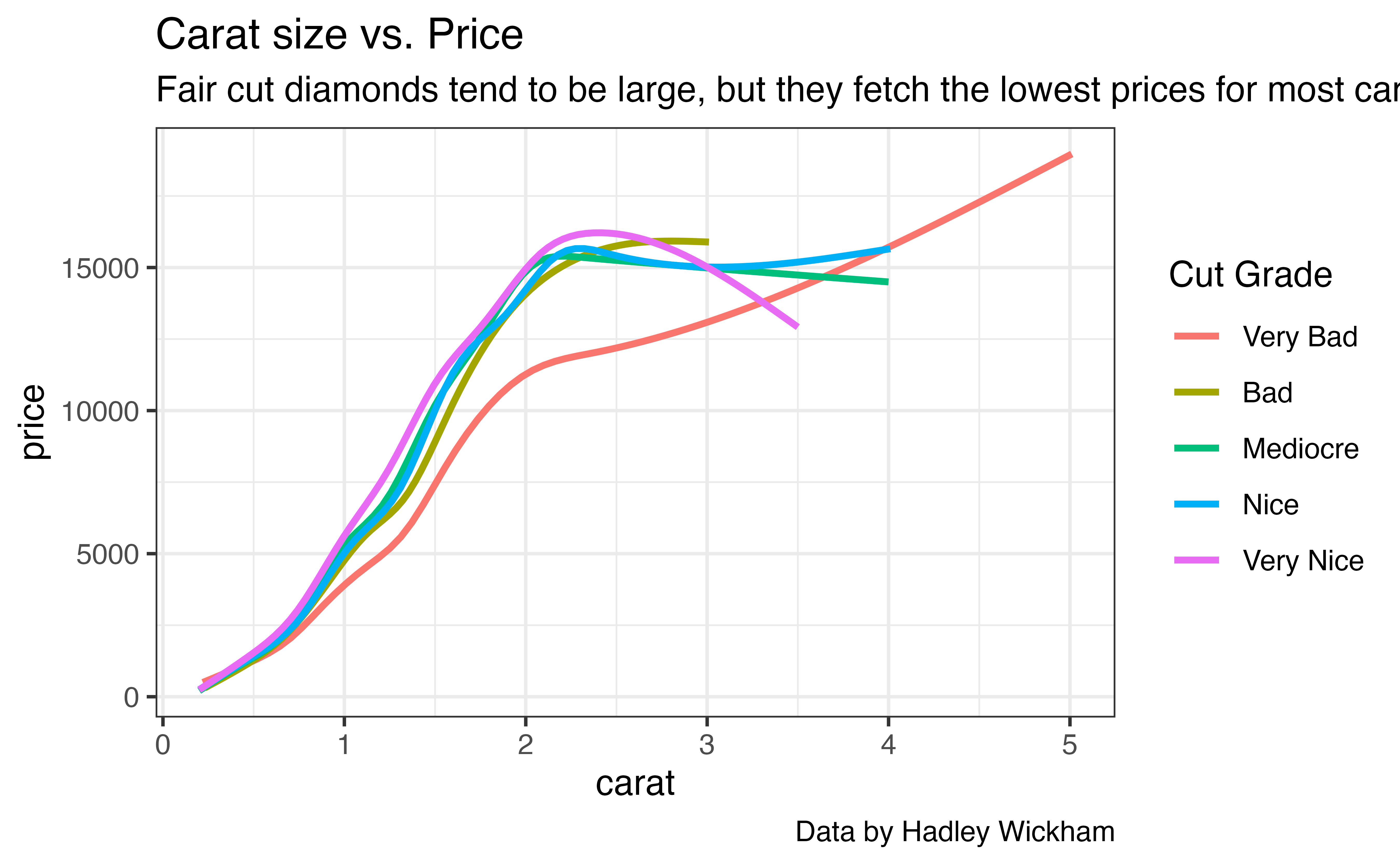
Exercise: guides()
Use guides() to remove each legend from the p_legend plot.
p_legend + guides(fill = "none", color = "none")Labels
To control the labels of a legend, you must turn to the scale_ functions. Each scale_ function takes a name and a labels argument, which it will use to build the legend associated with the scale. The labels argument should be a vector of strings that has one string for each label in the default legend.
So for example, you can adjust the legend of p1 with
p1 +
  scale_color_brewer(
    name = "Cut Grade",
    labels = c("Very Bad", "Bad", "Mediocre", "Nice", "Very Nice")
  )
What if?
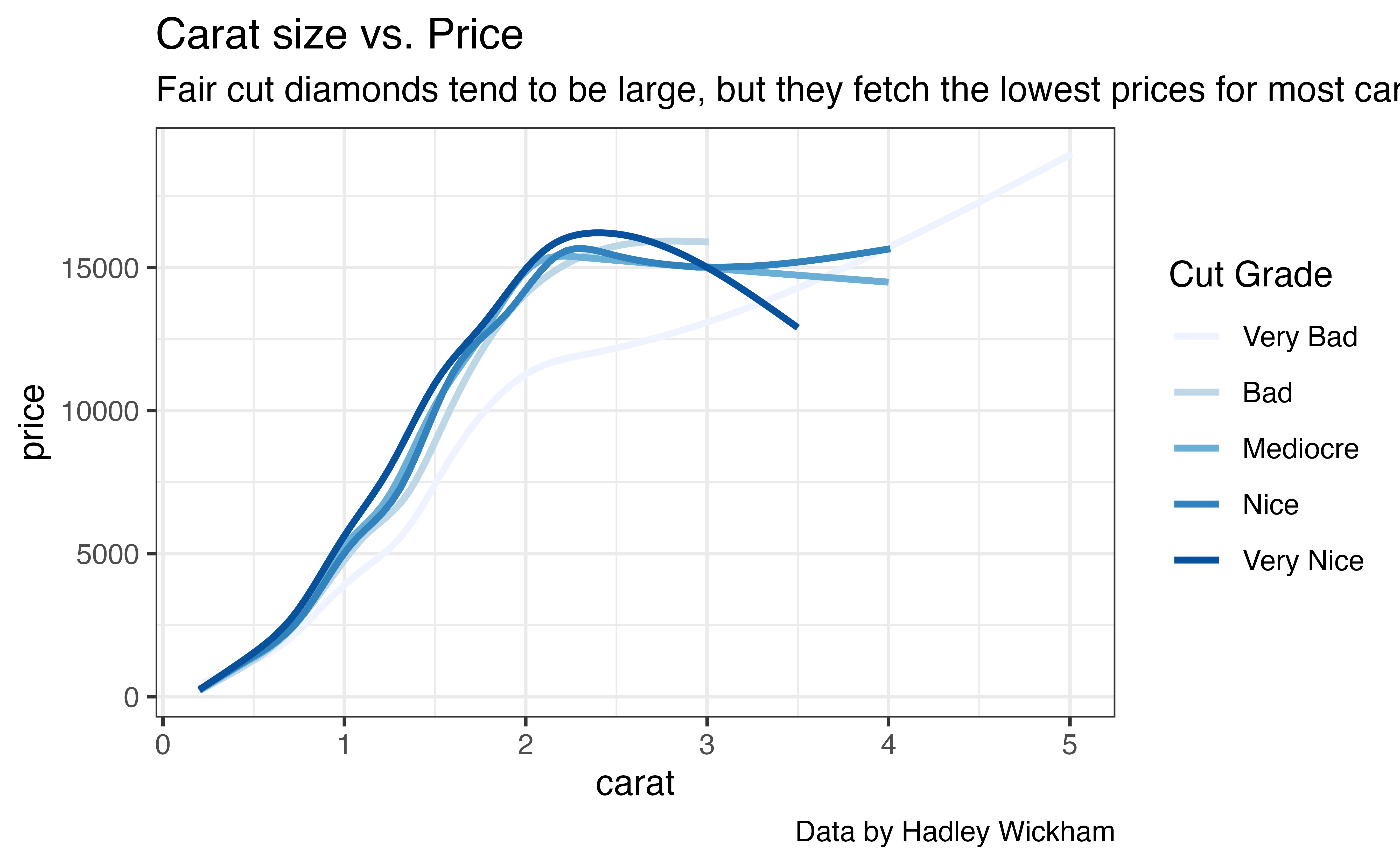
This is handy, but it raises a question: what if you haven’t invoked a scale_ function to pass labels to? For example, the graph below relies on the default scales.
Default scales
In this case, you need to identify the default scale used by the plot and then manually add that scale to the plot, setting the labels as you do.
For example, our plot above relies on the default color scale for a discrete variable, which happens to be scale_color_discrete(). If you know this, you can relabel the legend like so:
p1 +
  scale_color_discrete(
    name = "Cut Grade",
    labels = c("Very Bad", "Bad", "Mediocre", "Nice", "Very Nice")
  )
Scale defaults
As you can see, it is handy to know which scales a {ggplot2} graph will use by default. Here’s a short list.
| aesthetic | variable | default |
|---|---|---|
| x | continuous | scale_x_continuous() |
| discrete | scale_x_discrete() |
|
| y | continuous | scale_y_continuous() |
| discrete | scale_y_discrete() |
|
| color | continuous | scale_color_continuous() |
| discrete | scale_color_discrete() |
|
| fill | continuous | scale_fill_continuous() |
| discrete | scale_fill_discrete() |
|
| size | continuous | scale_size() |
| shape | discrete | scale_shape() |
Exercise: Legends
Use the list of scale defaults above to relabel the legend in p_cont. The legend should have the title “Highway MPG”. Also place the legend at the top of the plot.
p_cont +
  scale_color_continuous(name = "Highway MPG") +
  theme(legend.position = "top")

# This works too
p_cont +
  labs(color = "Highway MPG") +
  theme(legend.position = "top")
Good job!
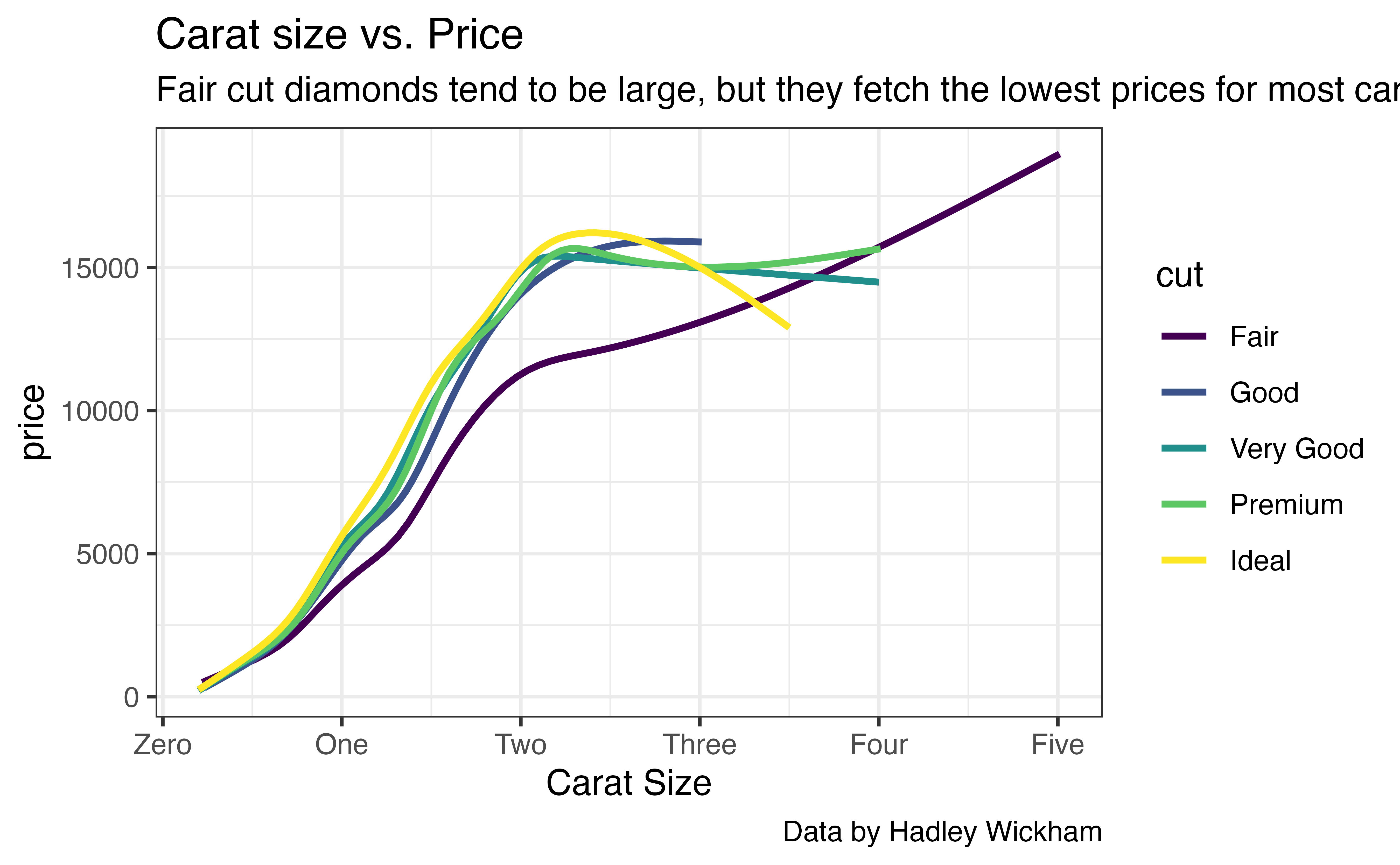
Axis labels
In {ggplot2}, the axes are the “legends” associated with the \(x\) and \(y\) aesthetics. As a result, you can control axis titles and labels in the same way as you control legend titles and labels:
p1 +
  scale_x_continuous(
    name = "Carat Size",
    labels = c("Zero", "One", "Two", "Three", "Four", "Five")
  )